Second-order Kinetics involving residual monomer in a dimerisation equilibrium

Scheme:

`2Astackrel(K_D)earrA_2`

`A+Bstackrel(k_1) rarrC`

Differential Equation:

`A'(t)=-k_1AB`

`B'(t)=-k_1AB`

`C'(t)=k_1AB`

Mass balance equation:

`A_0=A+2A_2+C`

`B_0=B+C`

Initial conditions:

`A(0)=A_0`, `B(0)=B_0` and `C(0)=0`

Full solution (pre-equilibrium assumption):

$$t = \ln \left( {{{\sqrt {8{K_D}\left( {{A_0} - C} \right) + 1} - 1} \over {\sqrt {8{K_D}\left( {{B_0} - C} \right)} }}} \right) + {{\sqrt {8{K_D}\left( {{B_0} - {A_0}} \right) - 1} } \over {{k_1}\left( {{A_0} - {B_0}} \right)}}\arctan \left( {{{\sqrt {8{K_D}\left( {{A_0} - C} \right) + 1} } \over {\sqrt {8{K_D}\left( {{B_0} - {A_0}} \right) - 1} }}} \right) - {c_1}$$

where,

$${c_1} = \ln \left( {{{\sqrt {8{K_D}{A_0} + 1} - 1} \over {\sqrt {8{K_D}{B_0}} }}} \right) + {{\sqrt {8{K_D}\left( {{B_0} - {A_0}} \right) - 1} } \over {{k_1}\left( {{A_0} - {B_0}} \right)}}\arctan \left( {{{\sqrt {8{K_D}{A_0} + 1} } \over {\sqrt {8{K_D}\left( {{B_0} - {A_0}} \right) - 1} }}} \right)$$

Approximate solution (pre-equilibrium assumption):

$$t = \frac{{8{K_D}}}{{{k_1}}}\frac{{\arctan \left( {\frac{{\sqrt {8{K_D}\left( {{A_0} - C} \right) + 1} }}{{\sqrt {8{K_D}\left( {{B_0} - {A_0}} \right) - 1} }}} \right)}}{{\sqrt {8{K_D}\left( {{B_0} - {A_0}} \right) - 1} }} + {c_2}$$

where,

$${c_2} = - \frac{{8{K_D}}}{{{k_1}}}\frac{{\arctan \left( {\frac{{\sqrt {8{K_D}{A_0} + 1} }}{{\sqrt {8{K_D}\left( {{B_0} - {A_0}} \right) - 1} }}} \right)}}{{\sqrt {8{K_D}\left( {{B_0} - {A_0}} \right) - 1} }}$$

Graph:

Note: As with other mechanisms which involve a single step, variation of the rate parameters does not affect the general form of the concentration-time curves obtained, with time scaled appropriately. However, the interactivity of the graph is to illustrate the how the approximate solution compares to the full solution. As described below, the approximation is valid for large K_D, however the approximation is fairly good for K_D>5.

Pre-amble

To solve this kinetic system we make use of the pre-equilibrium assumption. That is, we assume the equilibration between A and A₂ is extremely rapid on a comparitive time-scale to the irreversible reaction with B. That way we can treat the dimerisation equilibrium separately to the bimolecular rate process. Thus, we start off by expressing the concentration of A as it appears in the equilibrium `AearrA_2`. We then substitute this into the bimolecular rate expression, `C'(t)=k_1AB`, and solve the expression analytically. For the case of large Kd, we can approximate the expression with negligable loss of accuracy, but a large loss of complexity. The complete solution and the approximated solution are provided.

Derivation:

First following the derivation of the dimerisation equilibrium, we have,

`A=A_0-(4K_DA_0+1-sqrt(8K_DA_0+1))/(4K_D)`

However, this equilibrium expression is only true when the sum of `A` and `A_2` is constant, and in this case equal to A₀. For the case of this mechanism, `A` is depleted by an irreversible reaction, hence applying the pre-equilibrium assumption (assuming the rate of equilibration is significantly more rapid than the irreversible rate) we define the equilibrium in terms of the monomer and dimer. To do this we define a new mass-balance equation,

`A_Sigma=A+2A_2`

Replacing `A_0` with `A_Sigma` in the equilibrium expression we obtain,

`A=A_Sigma-(4K_DA_Sigma+1-sqrt(8K_DA_Sigma+1))/(4K_D)`

and

`A_2=(4K_DA_Sigma+1-sqrt(8K_DA_Sigma+1))/(8K_D)`

Using the equilibrium expression for `A(t)`, we can now solve the irreversible step. Using the differential equation `C'(t)`,

`C'(t)=k_1AB`

Substituting in the definition of `A` from the equilibrium,

`C'(t)=k_1(A_Sigma-(4K_DA_Sigma+1-sqrt(8K_DA_Sigma+1))/(4K_D))B`

Using the mass-balance equation, we express `A_Sigma` in terms of `C`,

`C=A_0-A-2A_2=A_0-A_Sigma` and so, `A_Sigma=A_0-C`

The rate expression becomes,

`C'(t)=k_1((A_0-C)-(4K_D(A_0-C)+1-sqrt(8K_D(A_0-C)+1))/(4K_D))B`

Next we need to express `B(t)` in terms of `C(t)`, which again we do using the mass-balance equation,

`B_0=B+C` and so `B=B_0-C`

Using this definition of `B`, we obtain the differential equation,

`C'(t)=k_1((A_0-C)-(4K_D(A_0-C)+1-sqrt(8K_D(A_0-C)+1))/(4K_D))(B_0-C)`

Which we can simplify to,

`C'(t)=k_1((1-sqrt(8K_D(A_0-C)+1))/(4K_D))(B_0-C)`

At this point we have the choice of solving the differential equation exactly, which we would achieve using integration by parts, or we can opt for an approximation.

Full Solution

The full, unapproximated solution is obtained through integration. Thus,

`t=(4K_D)/(k_1) int (dC)/((1-sqrt(8K_D(A_0-C)+1))(B_0-C))`

We arrive at a solution providing time as a function of C,

$$t = \ln \left( {\frac{{\sqrt {8{K_D}\left( {{A_0} - C} \right) + 1} - 1}}{{\sqrt {8{K_D}\left( {{B_0} - C} \right)} }}} \right) + \frac{{\sqrt {8{K_D}\left( {{B_0} - {A_0}} \right) - 1} }}{{{k_1}\left( {{A_0} - {B_0}} \right)}}\arctan \left( {\frac{{\sqrt {8{K_D}\left( {{A_0} - C} \right) + 1} }}{{\sqrt {8{K_D}\left( {{B_0} - {A_0}} \right) - 1} }}} \right) + {c_1}$$

where,

$${c_1} = - \ln \left( {\frac{{\sqrt {8{K_D}{A_0} + 1} - 1}}{{\sqrt {8{K_D}{B_0}} }}} \right) - \frac{{\sqrt {8{K_D}\left( {{B_0} - {A_0}} \right) - 1} }}{{{k_1}\left( {{A_0} - {B_0}} \right)}}\arctan \left( {\frac{{\sqrt {8{K_D}{A_0} + 1} }}{{\sqrt {8{K_D}\left( {{B_0} - {A_0}} \right) - 1} }}} \right)$$

Since we have now obtained an expression correlating time as a function of the concentration C, we now also express the other concentrations in the system, A and B, in terms of C. This is achieved using the mass-balance equations, thus,

`A_Sigma=A_0-C` and `C=B_0-C`

Approximate Solution

We just justify the use of an approximated form of the rate equation for the case of large K_D. This is possible since, in this case, `sqrt(8K_D(A_0-C)+1)" >> "1`. We make the simplification to the rate equation and arrive at,

`dt=(4K_D)/(k_1) (dC)/((-sqrt(8K_D(A_0-C)+1))(B_0-C))`

As before, the approximated solution is obtained through integration. Thus,

`t=(4K_D)/(k_1) int (dC)/((-sqrt(8K_D(A_0-C)+1))(B_0-C))`

Which has the solution,

where,

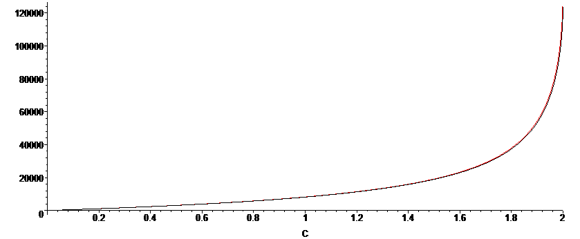
We can compare the accuracy for the two derived integrated rate expressions. We note that this formulation give time as a function of concentration C, hence we have time on the y-axis, and C on the x-axis, where A₀=2, B₀=2.1, k1=3x10^-3. As aforementioned, the validity of the approximation is most accurate when K_D is large, such that `sqrt(8K_D(A_0-C)+1)">>"1`, and with an equilibrium constant of K_D=1000, we observe a near perfect coincidence of the full, un-approximated solution (black) and the approximated solution (red).

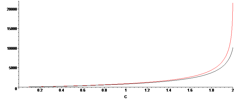
The approximation is less accurate for when K_D is smaller, as we can see in the plot below, for which K_D=10. There is still very good agreement when the reaction extent is less than 80%.

Derivation not finished...

A₀=2; B₀=2.1; k₁=3x10^-3
`K_D=`
graphing Kd=11