The Linear Approximation
Introduction
It is possible to construct from scratch the time-dependent evolution of concentrations in a kinetic using the numerical method, which involves approximating the changes in concentration that occur in time-steps as linear functions of time. Whilst it is not the case for the majority of reactions that changes are indeed linear, when small time-steps are employed, the accuracy improves until the point of an infinitesimal time-change when the linear approximation converges with the non-linear, exact solution. The approach involves often many hundreds of rows, and even more calculations to perform, and so we may wonder why this method interests us at all! Well, the answer lies in the fact that this approach can be applied to any kinetic system, irrelevent of mechanistic and algebraic complexity. As we've seen (here for instance), the exact solution for a complex mechanism can be surprisingly complex, when the solution even exists! In deed, many complex mechanisms actually lack any form of closed form solution and can often involve, even for mechanisms only minorly more convoluted than a single elementary process, transcendental special functions. Evidently, there are advantages to using the numerical solution, especially in solving intractable sets of differential equation and those for which the analytic solution elude us, but it is important to stress that, other than in exceptional circumstances, the numerical solution is always wrong! There is always a difference between the values approximated using the numerical method and the analytic solution.
The method of linear approximation involves calculating the change in concentrations that occur across small time-intervals ('bins'), and then adding these changes to the initial concentrations to provide an approximate figure for the concentrations at the beginning of the next time-interval. The process is repeated, until a complete profile is obtained.
Obviously, this approach requires a knowledge of the rate constants, in order to calculate the defintie changes. So the next question is, how do we employ this technique to analyse a reaction for which the rate constant is unknown - one of the most common tasks in kinetic analysis? The answer to this question involves taking an educated, ball-park figure guess for the rate constant, constructing the complete profile, and then varying the trial rate constants until the best fit with the experimental data is obtained. This naturally involves some form of estimation of goodness of fit, via a typical statistical analysis, least-squares regression for example.
Example I: Unimolecular Decay
Consider the Unimolecular Decay reaction,
`Astackrel(k)rarrB`
which has the kinetic differential equation,
`d/(dt)A=-kA`
and the mass balance,
`A_0=A+B`
We can construct the concentration-time evolution using the linear approximation, numerical solution. For example, we divide time up into intervals of 1000seconds. We make the linear assumption that during each 1000second interval, the definite change in concentration is,
`DeltaA=-kADeltat`
Which is equivalent to approximating the definite integral as a linear change,
`int dA=-k int Adt`
Thus in the first 1000 seconds, we have a change of, `DeltaA=-kA_0xx1000"seconds"`. To calculate the concentration of A at the beginning of the next time interval, we add this change (which we note is negative), to the concentration of A at the beginning of the last time interval. For this example, we have set `k=1xx10^(-4)s^(-1)`, and `A_0=2.1Mol`. Hence the change in the first 1000s is `DeltaA=-1xx10^(-4)s^(-1)xx2.1Molxx1000s=-0.21Mol`. We then add this change to the concentration at the beginning of the time interval, which gives us the concentration at the end of the first 1000s, ie., `A_(1000s)=A_0+DeltaA=2.1-0.21=1.89Mol`. Then in the next 1000s, we use the starting concentration of 1.89Mol, and as before calculate the definite change, `DeltaA=-1xx10^(-4)s^(-1)xx1.89Molxx1000s=-0.189Mol`, add this to the initial concentration of 1.89Mol and obtain the starting concentration for the next time interval, ie., `A_(2000s)=1.89-0.189=1.701Mol`. We repeat these calculations and produce a table:
| `t` | `A` | `DeltaA` | ||
| 0 | 2.1 | -0.21 | ||
| 1000 | 1.89 | -0.189 | ||
| 2000 | 1.701 | -0.1701 | ||
| 3000 | 1.5309 | -0.15309 | ||
| 4000 | 1.37781 | -0.13778 | ||
| 5000 | 1.240029 | -0.124 | ||
| 6000 | 1.116026 | -0.1116 | ||
| 7000 | 1.004423 | -0.10044 | ||
| 8000 | 0.903981 | -0.0904 | ||
| 9000 | 0.813583 | -0.08136 | ||
| 10000 | 0.732225 | -0.07322 | ||
| 11000 | 0.659002 | -0.0659 | ||
| 12000 | 0.593102 | -0.05931 | ||
| 13000 | 0.533792 | -0.05338 | ||
| 14000 | 0.480413 | -0.04804 | ||
| 15000 | 0.432371 | -0.04324 | ||
| 16000 | 0.389134 | -0.03891 | ||
| 17000 | 0.350221 | -0.03502 | ||
| 18000 | 0.315199 | -0.03152 | ||
| 19000 | 0.283679 | -0.02837 | ||
| 20000 | 0.255311 | -0.02553 |
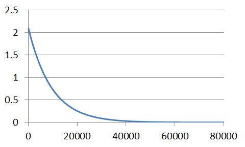
As we would expect, a graph of this series follows the exponential decay for a first-order process.

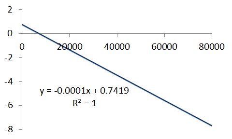
To illustrate the accuracy of our solution, we can handle the data as we would any other first-order process, ie., plot the logarithm of the concentrations against time - a first-order process reveals a linear function.
| `t` | `A` | `DeltaA` | ||
| 0 | 2.1 | 0.741937 | ||
| 1000 | 1.89 | 0.636577 | ||
| 2000 | 1.701 | 0.531216 | ||
| 3000 | 1.5309 | 0.425856 | ||
| 4000 | 1.37781 | 0.320495 | ||
| 5000 | 1.240029 | 0.215135 | ||
| 6000 | 1.116026 | 0.109774 | ||
| 7000 | 1.004423 | 0.004414 | ||
| 8000 | 0.903981 | -0.10095 | ||
| 9000 | 0.813583 | -0.20631 | ||
| 10000 | 0.732225 | -0.31167 | ||
| 11000 | 0.659002 | -0.41703 | ||
| 12000 | 0.593102 | -0.52239 | ||
| 13000 | 0.533792 | -0.62775 | ||
| 14000 | 0.480413 | -0.73311 | ||
| 15000 | 0.432371 | -0.83847 | ||
| 16000 | 0.389134 | -0.94383 | ||
| 17000 | 0.350221 | -1.04919 | ||
| 18000 | 0.315199 | -1.15455 | ||
| 19000 | 0.283679 | -1.25991 | ||
| 20000 | 0.255311 | -1.36527 |
Here's a plot of lnA, for the data generated using the linear approximation, with Excel's linear regression parameters. Comparison of the equation of the straight-line to the logarith of the time-dependence of A, illustrates which parameters are of particular interest, ie.,
`lnA=lnA_0-kt`
and reveals the gradient of the line is the negative rate constant. The analysis below provides a rate constant of `1xx10^(-4)`, as we expected, in agreement with that we used to generate the series.

Example II: Elementary Bimolecular Mechanism
Consider the Bimolecular reaction,
`A+Bstackrel(k)rarrC`
which has the kinetic differential equation,
`d/(dt)A=-kAB`
and the mass balance,
`A_0=A+C` and `B_0=B+C`
Using the same method as example I, we construct the concentration-time evolution by dividing time up into intervals of 1000seconds. We make the linear assumption that during each 1000second interval, the definite change in concentration is,
`DeltaA=-kABDeltat`
As before, we calculate the change for each interval based on the concentration values at the start of each interval, add the change to the initial concentration and carry that down to the initial concentration of the next time interval. For this simulation, we use the values, `A_0=2.1`, `B_0=3.1`, `C_0=0` and `k=5xx10^(-5)`.
| `t` | `A` | `B` | `C` | `DeltaAB` | ||||
| 0 | 2.1 | 3.1 | 0 | -0.3255 | ||||
| 1000 | 1.7745 | 2.7745 | 0.3255 | -0.24617 | ||||
| 2000 | 1.528332 | 2.528332 | 0.571668 | -0.19321 | ||||
| 3000 | 1.335126 | 2.335126 | 0.764874 | -0.15588 | ||||
| 4000 | 1.179242 | 2.179242 | 0.920758 | -0.12849 | ||||
| 5000 | 1.050749 | 2.050749 | 1.049251 | -0.10774 | ||||
| 6000 | 0.943008 | 1.943008 | 1.156992 | -0.09161 | ||||
| 7000 | 0.851394 | 1.851394 | 1.248606 | -0.07881 | ||||
| 8000 | 0.772581 | 1.772581 | 1.327419 | -0.06847 | ||||
| 9000 | 0.704108 | 1.704108 | 1.395892 | -0.05999 | ||||
| 10000 | 0.644114 | 1.644114 | 1.455886 | -0.05295 | ||||
| 11000 | 0.591164 | 1.591164 | 1.508836 | -0.04703 | ||||
| 12000 | 0.544132 | 1.544132 | 1.555868 | -0.04201 | ||||
| 13000 | 0.502122 | 1.502122 | 1.597878 | -0.03771 | ||||
| 14000 | 0.464409 | 1.464409 | 1.635591 | -0.034 | ||||
| 15000 | 0.430405 | 1.430405 | 1.669595 | -0.03078 | ||||
| 16000 | 0.399622 | 1.399622 | 1.700378 | -0.02797 | ||||
| 17000 | 0.371656 | 1.371656 | 1.728344 | -0.02549 | ||||
| 18000 | 0.346167 | 1.346167 | 1.753833 | -0.0233 | ||||
| 19000 | 0.322867 | 1.322867 | 1.777133 | -0.02136 | ||||
| 20000 | 0.301512 | 1.301512 | 1.798488 | -0.01962 |
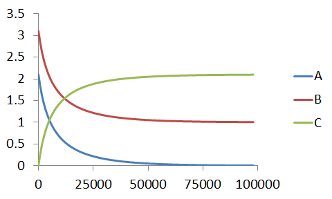
Using these values we obtain the following concentration-time profile - it certainly looks like a bimolecular profile, but is it?

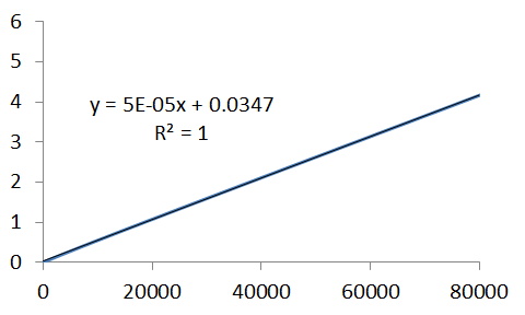
If our linear approximation is valid, then we should be able to analyse it as such. As per the solution detailed here, we can analyse the data using the characteristic equation,
`kt=1/(A_0-B_0) [ln((A_0-C_t)/A_0) - ln((B_0-C_t)/B_0)]`
which gives a straight line only if the kinetics exactly match the bimolecular case.
| `t` | characteristic equation | |
| 0 | 0 | |
| 1000 | 0.057487 | |
| 2000 | 0.113918 | |
| 3000 | 0.169575 | |
| 4000 | 0.224641 | |
| 5000 | 0.279237 | |
| 6000 | 0.333453 | |
| 7000 | 0.387354 | |
| 8000 | 0.44099 | |
| 9000 | 0.494401 | |
| 10000 | 0.547616 | |
| 11000 | 0.600663 | |
| 12000 | 0.65356 | |
| 13000 | 0.706327 | |
| 14000 | 0.758976 | |
| 15000 | 0.811522 | |
| 16000 | 0.863973 | |
| 17000 | 0.91634 | |
| 18000 | 0.96863 | |
| 19000 | 1.020851 | |
| 20000 | 1.073008 |
Once we have plot our characteristic equation, once again, we interpret the gradient as the rate constant, which as expected, is in perfect agreement with that used to generate the simulated data.
