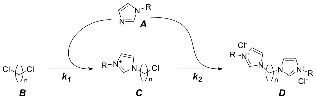
Parallel-Consecutive Second-order Kinetics
- Preamble
- Outline of the Procedure
- Setting up the Differential Equations
- Solutions expressing concentration to concentration
- Expressing a Correlation with Time
- Evaluating the Lerch Transcendent
Scheme:
`A+Bstackrel(k_1) rarrC`
`A+Cstackrel(k_2) rarrD`
for example,
Differential Equations:
|
`A'(t)=-k_1AB-k_2AC` `B'(t)=-k_1AB` `C'(t)=k_1AB-k_2AC` `D'(t)=k_2AC` |
Case I: A0 = 2B0 AND k2/k1≠1≠2
Mass Balance:
`A_0=A+C+2D`
`B_0=B+C+D`
`A_0/B_0=2`
Hence, `C=A-2B`
Some specific defintions
To make the equations easier to manipulate we make use of the following substitutions,
`alpha=A/A_0`, `beta=B/B_0`, `gamma=C/B_0`, `delta=D/B_0`, `kappa=k_2/k_1` and `d tau=B_0k_1dt`
The foremost four of these (`alpha, beta, gamma, delta`) are fractional concentrations - that is, they represent the concentration as a fraction of its maximum. The use of fractional concentrations can be useful to frame the solutions of the kinetic equations within the limits of [conc]=0..1. Otherwise, we have variable limits which will complicate the solution. The latter two substitutions (`kappa` and `tau`) enable further simplification of the differential equations.
Solution:
`alpha(beta)=A_0((1-2kappa)beta+beta^kappa)/(2(1-kappa))`
`gamma(beta)=(beta^kappa-beta)/(1-kappa)`
`delta(beta)=1+(kappabeta+beta^kappa)/(1-kappa)`
`t = (z beta^(-1) Phi(beta^(kappa-1)/(2kappa-1),1,1/(1-kappa))- z Phi(1/(2kappa-1),1,1/(1-kappa)))/(k_1B_0)`
Nb: `Phi(...)` is the Lerch Transcendent
Graph:
The set of differential equations are non-linear and constitute an intractable set, which does not have an exact solution, ie., the set is not separable nor do they conform to a standard form. Instead, we have to solve them as a set of equations simultaneous in time. This has the unfortunate consequence that whilst it is possible to provide exact expressions relating the concentrations A, B, C and D to one another, it is not possible to exactly express their time-dependance. It is however possible to correlate time with concentrations with an approximate expression.
We take the set of differential equations, convert them to a form involving fractional concentrations, and replace time with scaled time, `tau`. Next we convert these non-linear time-differential equations into linear-differential equations by eliminating 'time' by dividing each by `beta'(tau)`. We solve the new set of linear differential equations to provide expressions relating the concentrations to one-another. Using these solutions, we then formulate an expression to recover time, which involves a single intractable integral (which is easier than solving a set of four intractable differential equations!) - this expression is only an approximation of time, but one which can provide an arbitrary accuracy.
Setup the differential equations in `tau` basis
Convert the diffferential equation `A'(t)` and `B'(t)` to `alpha'(tau)` and `beta'(tau)` using the substitutions `beta=B_0B` and `alpha=A_0A`:
`B'(t)=-k_1AB=-k_1A_0B_0alphabeta=B_0(d beta)/(dt)`
Hence,
`(d beta)/(k1B_0dt)=(d beta)/(d tau)=-2alphabeta`
Then we do the same for the equation `A'(t)`. First we substitute in the definition of `C` from the mass balance equation,
`A'(t)=-k_1AB-k_2A(A-2B)=(2k_2-k_1)AB-k_2A^2`
Next substitute in the definitions for fractional concentrations,
`A_0(dalpha)/(dt)=(2k_2-k_1)A_0B_0alphabeta-k_2A_0^2alpha^2`
...and substitute in the definitions of `kappa=k_2/k_1` and `d tau=k_1B_0dt`,
`(dalpha)/(B_0k_1dt)=(dalpha)/(d tau)=(2kappa-1)alphabeta-2kappaalpha^2`
This differential equation `alpha'(tau)` can be made linear by dividing it `beta'(tau)`,
`(dalpha)/(d tau) (d tau)/(dbeta)=((2kappa-1)alphabeta)/(-2alphabeta)-(2kappaalpha^2)/(-2alphabeta)`
Which becomes the linear first order differential eqation,
`(dalpha)/(dbeta)=kappa alpha/beta + (1-2kappa)`
The solutions of `alpha`, `gamma` and `delta` in terms of `beta`
The solution to this can be found by either using u-substitution with `w=kappa alpha/beta` or the integrating factor method. To solve it we here use the former method. First we define,
`m=(1-2kappa)/2` and `w=kappa alpha/beta`
So the equation becomes,
`(dalpha)/(dbeta)=w+m`
We solve w for `alpha` and differentiate,
`alpha=1/kappa w beta`, `(d alpha)/(dbeta)=1/kappa (w + beta(dw)/(dbeta))`
Which leads to,
`(dalpha)/(dbeta)=w+m=1/kappa (w + beta(dw)/(dbeta))`
Multiplying by `kappa`,
`kappaw+kappam=w + beta(dw)/(dbeta)`
Subtract w from both sides,
`(kappa-1)w+kappam=beta(dw)/(dbeta)`
Now we again use u-substitution, this time we define `u=(kappa-1)w+kappam`, and obtain the derivative,
`(du)/(dw)=(kappa-1)` and `(du)/(kappa-1)=dw`
We substitute u back into the equation, and then the expression `dw` just obtained,
`u=beta(dw)/(dbeta)=beta/(dbeta) (du)/(kappa-1)`
This equation is now separable and so we can integrate,
`(kappa-1) int(dbeta)/beta=int(du)/u`
...to obtain,
`(kappa-1)lnbeta=lnu +c_1`
We reverse the substitution u and then w,
`(kappa-1)lnbeta=ln ((kappa-1)w+kappam) +c_1=ln ((kappa-1)kappa alpha/beta +kappam) +c_1`
Using the particular value `alpha(1)=1` we can find the integration coefficient,
`0=ln ((kappa-1)kappa +kappam) +c_1`
`-c_1=ln ((kappa-1)kappa +kappam)`
`exp(-c_1)=(kappa-1)kappa+kappam`
Returning to the solution, we exponentiate it and move the integration coefficient to the l.h.s.,
`beta^(kappa-1)exp(-c_1)=(kappa-1)kappa alpha/beta +kappam`
Multiply both sides by `beta`, and subtract the m term,
`beta^(kappa)exp(-c_1)-kappambeta=(kappa-1)kappa alpha`
Solve for `alpha`
`alpha=(kappambeta-beta^(kappa)exp(-c_1))/((1-kappa)kappa)`
Substitute in the definition of `exp(-c_1)`, and cancel the common `kappa` terms,
`alpha=(mbeta-beta^(kappa)((kappa-1)+m))/((1-kappa))`
Recall our definition of m, and substitute this in,
`alpha=(((1-2kappa)/2)beta-beta^(kappa)((kappa-1)+((1-2kappa)/2)))/((1-kappa))`
Expand the brackets and factorise the numerator for a factor of 2,
`alpha=((1-2kappa)beta-2(kappa-1)beta^kappa-(1-2kappa)beta^kappa)/(2(1-kappa))`
Expand the `beta^kappa` terms,
`alpha=((1-2kappa)beta-2kappabeta^kappa+2beta^kappa-beta^kappa+2kappabeta^kappa)/(2(1-kappa))`
We cancel the common terms and finally obtain,
`alpha(beta)=((1-2kappa)beta+beta^kappa)/(2(1-kappa))`
Using this solution to the `alpha'(beta)` differential equation, it is possible through the various mass balance equations to find expressions for the other concentrations, `gamma` and `delta`. We take the mass balance equations and convert them to fractional concentrations,
| `B_0=B+C+D` | → | `1=beta+gamma+delta` |
| `C=A-2B` | → | `gamma=2alpha-2beta` |
Substituting in the solution `alpha(beta)` into the above mass balance equations, and we obtain,
`gamma(beta)=(beta^kappa-beta)/(1-kappa)` and `delta=1-beta-(beta^kappa-beta)/(1-kappa)`
Expressing a Correlation with Time
Having removed the time dependance from the differential equations in order to make them linear and exactly solvable, we now need to obtain a mean to correlate these concentrations with time. To do this, we take a time-differential equation which is separable, the simplest of which being `beta'(tau)`, and integrate. Recall the definition,
`beta'(tau)=-2alphabeta`
Replace `alpha` with the solution previously derived,
`beta'(tau)=(d beta)/(d tau)=-((1-2kappa)beta^2+beta^(kappa+1))/(1-kappa)`
Factorise for -1,
`(d beta)/(d tau)=((2kappa-1)beta^2-beta^(kappa+1))/(1-kappa)`
Reciprocate the equation, separate the variables and integrate,
`int_0^L (d beta)/((2kappa-1)beta^2-beta^(kappa+1))=int (d tau)/(1-kappa)`
This integral is intractable (it cannot be expressed in a finite number of terms of elementary functions ie., does not have a closed form), however we can approximate it to an arbitrary accuracy using the Lerch-Transcendent function. Compare the above integral to both the integrals below,
The Hypergeometric Euler integral,
`I=int_0^1 ((1-u)^(g-f-1)u^(f-1)du)/(1-ux)^e=(Gamma(g-f)Gamma(f))/(Gamma(g)) ""_2F_1(e,f;g;x)`
...and also the integral representation of the Lerch-Transcdenent function
`I=int_0^1 (u^(a-1)(du))/(1-ux)=Phi(x,1,a)`
To make our integral conform to these, we factorise it for `(2kappa-1)beta^2` to obtain,
`int (d tau)/(1-kappa)=(2kappa-1)^(-1) int_0^L (beta^(-2)d beta)/(1-(2kappa-1)^(-1)beta^(kappa-1))`
Let `z=(2kappa-1)^(-1)`, then
`int (d tau)/(1-kappa)=z int_0^L (beta^(-2)d beta)/(1-zbeta^(kappa-1))`
We need to change the limits of integration which can we using u-substitution, let `w=beta/L` and so `(dLw)/(dbeta)=1`. Inserting these definitions to the integral we obtain,
`int (d tau)/(1-kappa)=z int_0^1 ((Lw)^(-2) d(Lw))/(1-z(Lw)^(kappa-1))`
Then we expand the brackets and collect the L terms,
`int (d tau)/(1-kappa)=z L^(-1) int_0^1 (w^(-2) dw)/(1-zL^(kappa-1)w^(kappa-1))`
Next we perform another u-substitution, this time `u=w^(kappa-1)`, and `(du)/(dw)=(kappa-1) w^(kappa-2)` so `dw=w^(2-kappa)/(kappa-1)du`, and obtain,
`int (d tau)/(1-kappa)=z L^(-1)/(kappa-1) int_0^1 (w^(-2) w^(2-kappa)du)/(1-zL^(kappa-1)u)`
We cancel the common terms, and express `w^(-kappa)` in terms of u, using `u^(1/(kappa-1))=w` we have `w^(-kappa)=u^(kappa/(1-kappa))`, and so,
`-int d tau=z L^(-1) int_0^1 ( u^(kappa/(1-kappa)) du)/(1-zL^(kappa-1)u)`
This integral now is of the Euler form, viz.,
`Phi(x,1,a)=int_0^1 (u^(a-1)(du))/(1-ux) = int_0^1 ( u^(kappa/(1-kappa)) du)/(1-zL^(kappa-1)u)`
From inspection we have,
`a-1=kappa/(1-kappa)`
Thus the integral can be expressed using the Lerch transcendent using:
`a=1/(1-kappa)`, and `x=L^(kappa-1)/(2kappa-1)`.
Hence,
`-int (d tau)/(1-kappa)=z int_0^L (beta^(-2)d beta)/(1-(2kappa-1)^(-1)beta^(kappa-1))=z L^(-1) Phi(L^(kappa-1)/(2kappa-1),1,1/(1-kappa))`
To make the integral useful, we need to change the limits again as to represent the time taken for `beta` to drop from 1 to L, rather than 0 to L. So we split the integral,
| `int_0^1...=int_0^L...+int_L^1...` |
We are interested in the integral of `beta=1..L` which corresponds to `tau|_0^beta`,
`-tau_beta = int_L^1=int_0^1-int_0^L`
Using our definition in terms of the Lerch function, we finally arrive with an expression to give time from a concentration,
`tau_beta = z L^(-1) Phi(L^(kappa-1)/(2kappa-1),1,1/(1-kappa))- z Phi(1/(2kappa-1),1,1/(1-kappa))`
Recalling our specific definition for scaled time, `tau=k_1B_0t`, we convert scaled time to time in seconds by dividing `tau` by `k_1B_0`.
As previously alluded to, the time-integral is intractable, which means it cannot be evaluated through an expression with a finite number of terms. However, the solution can be approximated through what is comparable to a series expansion. As described on this page, the Lerch Transcendent can be evaluated using the following infinite series,
`Phi(z,s,a)=sum_(n=0)^oo z^n/(a+n)^s`
In a form relevent to the parallel consecutive bimolecular mechanism, `s=1`.