Solving a Kinetic System as a set Simultaneous in time
- Motivation
- Example I: (regular concentrations) Two-step Consecutive First-Order
- Example II: (reduced concentrations)
Motivation
Sometimes the differential equations are not solvable analytically because there are too many inter-dependant variables. So we solve the concentratiosn relative to one another, which may have an exact analytic solution, and then we just need to correlate the concentrations with time. For the purpose of illustration, we have worked through the example below (Two-step Consecutive First-Order mechanism) - in that case, it is not an absolute necessity to to solve the equations as a simultaneous set. For an example where this method is necessary, see the parallel-consecutive bimolecular mechanism.
Example I: (Regular Concentrations) Two-step Consecutive First Order
`Astackrel(k_1) rarrB stackrel(k_2) rarrC`
Differential Equations
|
`A'(t)=-k_1A` `B'(t)=k_1A-k_2B` `C'(t)=k_2B` |
Mass balance equation
`A_0=A+B+C`
Initial conditions:
`A(0)=A_0`, `B(0)=0` and `C(0)=0`
We divide each of the differential equations by one of the most simple ones. In this case, we choose to divide by `A'(t)`. If we introduce the ratio rate constant, `kappa=k_2/k_1`, and also replace B with its definition from the mass balance equation from the differential equation `C'(A)` we obtain,
Simultaneous in time, Differential Equation
`B'(A)=k_2/k_1 B/A-1=kappa B/A-1`
Which has the solution,
`B(A)=c_1A^kappa-A/(1-kappa)`
Where the initial conditions require, `0=c_1A_0^kappa-A_0/(1-kappa)`, which gives, `c_1=A_0^(1-kappa)/(1-kappa)`
So the solution for B, is,
`B(A)=A_0^(1-kappa)/(1-kappa)A^kappa-A/(1-kappa)`
Then using the mass balance relationship we can express C,
`C=A_0-A-B=A_0-A-A_0^(1-kappa)/(1-kappa)A^kappa-A/(1-kappa)`
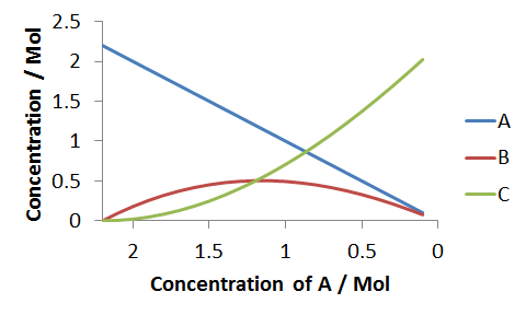
So to construct the full reaction evolution, we tabulate a range of A concentrations, ranging from A0 and 0, then using the full above, express B and C in terms of A. From this, we can construct a plot, showing A, B and C as a function of A. So the next step is to correlate the concentrations with time. To do this, we take the most simple time-differential equation, and reciprocate it, making `dt` the subject. Upon integration we obtain an expression that provides time as a function of a concentrations, ie.,
Starting with the differential equation, `A'(t)`,
`(dA)/(dt)=-k_1A`
Solve it for `dt`,
`dt=-1/k_1 (dA)/(A)`
We set-up the expression for integration,
`t=-1/k_1 int_A^(A_0) (dA)/(A)`
note the limits that we have used. We want to calculate the time taken for the concentration of starting material to drop from its initial value, A0, to some arbitrary final value, A. We can now evaluate the integral,
`t=-1/k_1 [ln A]_A^(A_0)`
`t=(lnA_0-ln A)/k_1 `
As described, we first tabulate a series of values of A, from A0 to 0.1 (we dont go to 0, since the reaction can take orders of magnitude much longer to come to arbitrarily close to completion). Then using the solutions `B(A) and C(A)`, we obtain values for the other concentrations. For this simulations we've used the parameters, `A_0=2.2Mol`, `kappa=2.3` and `k_1=1xx10^(-5)s^(-1)`,

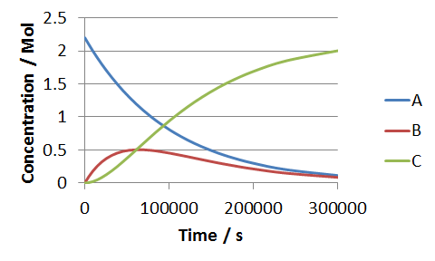
Next we have to calculate a series of time values that we can correlate against the concentrations. We do this by using the the time correlation equation, `t=(lnA_0-ln A)/k_1 `, which like B and C, we generate as a function of A. Now we can plot the three concentrations against the newly evaluated values of time.

What we find, is that the concentration-time profiles generated exactly match those calculated using the exact solution to the time-differential equations. Evidently, for the case of this mechanism, the method of solving the kinetic equations simultaneous in time was not a necessary step to solving the system, but it illustrates the procedure perfectly, and provides results that you can check against the values obtained using the complete solution (ibid). For this particular mechanism, the time-correlation equation involves an easily evaluated integral, however this is not always the case, as we found for the parallel-consecutive bimolecular mechanism. Hopefully something, too, that this example has demonstrated, is the advantage of working in fractional concentrations - all the terms involving A0 would be combined into their respective fractional concentrations, and all of the `A_0^x` would become unity.