Kinetic Linearisation via Definite Integrals

For some particularly convoluted mechanisms, it is not always (even often) possible to find analytic expressions for the integrated rate equations, and so to analyse the data, 'solving the inverse problem' we have to use numerical methods. Whilst it is possible to model the data using the numerical linear approximation method and perform a least-squares non-linear regression, an arguably more direct approach is to linearise the experimental data via graphical integration. Certainly, less calculations are required for this latter technique.

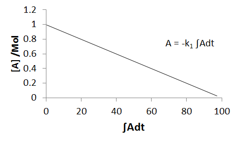
The objective of kinetic linearisation is to by some means linearise the progression of the chemical reaction, like is done when analysing first and second-order reactions (using the logarithmic and the reciprocal plots respectively), and then access the rate constants which are interpretted from the gradient. If we consider the kinetic equations for any chemical process, upon integration we obtain expressions for the changes in concentrations.

`d/(dt)A=-kA`

 Whilst it is often desirable to find a closed form expression of the evaluation, we do not have to. Instead, we can leave the integrals un-evaluated,

`DeltaA=-k int Adt`

If we then obtain the integral numerically, by treating the a plot of A against time graphically and calculating the area-under-curve, we have values for both sides of the equation. If we now plot `DeltaA`, ie., `A-A_0`, against the integral `int Adt`, we obtain a straight line with a gradient equal to `-k`. 

Due to the cumulative nature of numerical integration, errors become compounded. Additionally, the accuracy of the integral depends strongly upon the number and frequency of measurements - naturally, when we have very frequent measurements, the accuracy is at its best. At the other extreme, with only a single datapoint (other than zero), we are effectively approximation to the complete reaction profile as being a linear function - which is it not.

Example I: The three-step Parallel-Consecutive Bimolecular Mechanism

For example, the reaction of trisodium triimesate with propyl chloride.

Consider the three-step parallel-consecutive bimolecular mechanism,

`A+Bstackrel(k_1)rarrC`

`A+Cstackrel(k_2)rarrD`

`A+Dstackrel(k_3)rarrE`

Using some example data, for example from an experiment (`A_0=3.3, B_0=1.1,C_0=D_0=E_0=0`), we have the following time-concentration profiles,

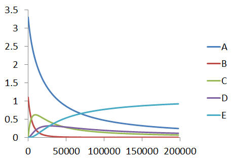
The mechanism has the kinetic equations,

`d/(dt) A=-k_1AB-k_2AC-k_3AD` `d/(dt) B=-k_1AB` `d/(dt) C=k_1AB-k_2AC` `d/(dt) D=k_2AC-k_3AD` `d/(dt) E=k_3AD`

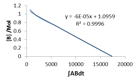
To analyse the data by linearisation, we need evaluate, numerically, some of the concentration products on the right hand side. We start with the simplest of the differential equation, `B'(t)`, we integrate by time,

`DeltaB=-k_1int ABdt`

We then plot `DeltaB` ie., `B-B_0`, against `int ABdt`, and this gives a straight line with a gradient of -k₁.

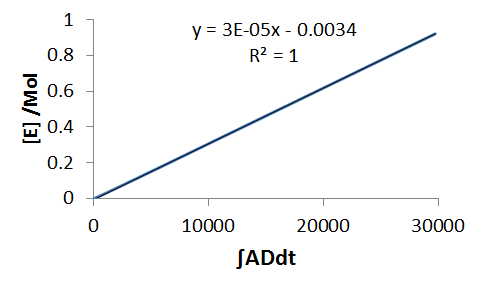
Next we do the same for the equation, `E'(t)` - solve for dE and integrate,

`DeltaE=k_3 intADdt`

Hence from a plot of `DeltaE` (since E₀=0, then `DeltaE=E`) against the integral `int ADdt` we obtain, as the gradient, the rate constant k₃.

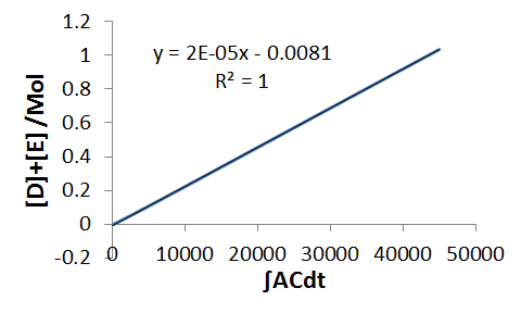
Access to the next rate constants involves manipulating the longer differential equation, those involving two terms. In order for them to yield straight lines, we need to arrange the equations with concentrations as functions of one individual integral. Next we will obtain the rate constant k₂ from the kinetic equation `D'(t)`, as before, we integrate it,

`DeltaD=k_2 int ACdt -k_3 intADdt`

We note that the value of certain integrals are equal changes in certain concentration, consider the appear of the term `k_3 intADdt`, which we recognise as the concentration change, `DeltaE`. We substitute this in,

`DeltaD=k_2 int ACdt -DeltaE`

Adding this to both sides, we now have a function we can plot against the remaining integral,

`DeltaD+DeltaE=k_2 int ACdt`

Since `D_0=E_0=0` then we have,

`D+E=k_2 int ACdt`

Hence we now have values for each of the rate constants,

`k_1=6xx10^(-5) Mol^(-1)s^(-1)`

`k_2=2xx10^(-5) Mol^(-1)s^(-1)`

`k_3=3xx10^(-5) Mol^(-1)s^(-1)`

and these are indeed the authentic rate constants.